While exploring the remains of a downed Star Destroyer, Han Solo and Rey are detected by a platoon of storm troopers. This rogue Imperial remnant intends to capture Han and Rey if possible, or terminate them otherwise. Our heroes, cornered in the hangar of the decrepit starship, see the soldiers approaching their position and consider their options.
Rey realizes the odds of them out-gunning their adversaries are grim. Han is the only one with a blaster, and she assumes his accuracy is roughly 50%. Having never seen Han in a fight before, 50% accuracy seems like a fair assumption.
|
1 |
accuracy <- 0.50 |
|
1 |
accuracy = 0.50 |
But with 30 storm troopers closing in fast, Han would likely need a much higher accuracy to take them all out before he and Rey are overwhelmed. Recognizing this, Rey insists they make a run for it. Han replies they’d never make it back to the Falcon before the soldiers catch up with them, and that they have no choice but to stand their ground. Besides, he says, he may be old, but he’s still the best shot in the star system. For both our sakes, I hope you aren’t just bluffing, says Rey. Trust me kid, I’ve got it when it counts, replies Han.
The storm troopers have split up into groups of 10, and the first group charges into the hangar. The troopers are some distance away yet and sprinting, so their shots are wild, but Han knows he needs to take them out before they can close the gap. Alternating between shooting and ducking behind old crates and engine parts, Han gets off 10 shots, 8 of which hit their mark. The two surviving storm troopers perform a quick mental calculation decide to advance in the opposite direction.
|
1 2 3 4 5 |
hit <- 1 miss <- 0 shots <- c(rep(hit, 8), rep(miss, 2)) print(shots) |
|
1 2 3 4 5 |
hit = 1 miss = 0 shots = [hit]*8 + [miss]*2 print(shots) |
|
1 |
1 1 1 1 1 1 1 1 0 0 |
|
1 |
[1, 1, 1, 1, 1, 1, 1, 1, 0, 0] |
Peering from behind a rusted turbine as Han blows at his blaster barrel’s smoke, Rey sees the 8 dead troopers scattered across the area and wonders to herself if Han’s accuracy is actually higher than 50%. Certainly, his accuracy was higher than 50% just now.
|
1 2 |
## calculate Han's accuracy, or average hit rate, for the first group mean(shots) |
|
1 2 |
## calculate Han's accuracy, or average hit rate, for the first group float(sum(shots))/len(shots) |
|
1 |
0.8 |
|
1 |
0.8 |
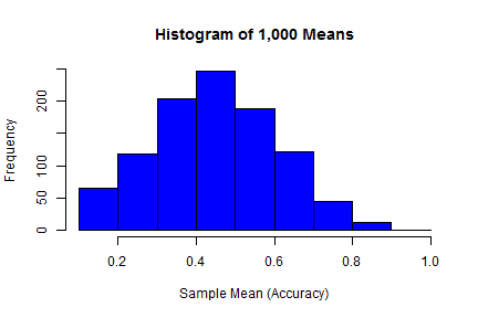
But is that impressive display sufficient evidence to say that Han’s accuracy, in the long run, is actually higher than 50%? Or was his sharp-shooting simply a chance fluctuation? Rey pulls out her computer and, being a Jedi Programmer in both R and Python, performs a quick simulation.
|
1 2 3 4 5 6 7 8 9 10 11 12 13 14 15 16 17 18 19 20 21 22 23 24 25 26 27 28 29 30 31 32 33 34 35 36 |
## Let's pretend that we know Han's accuracy is 50% ## and let's also randomly generate 10,000 shots numberOfShots <- 10^4 ## set the seed so we can reproduce our results set.seed(162534) ## sample() allows us to simulate 10,000 shots based on Han's accuracy ## x is the stuff our sample can be made of ## replace = TRUE makes sure we can have more than just one hit or miss ## prob is the probability of hit and miss, respectively (both 0.50) simulatedShots <- sample(x = c(hit, miss), size = numberOfShots, replace = TRUE, ## remember accuracy is 0.50 prob = c(accuracy, 1-accuracy)) ## organize the 10,000 shots into 1,000 groups of 10 shots with a matrix groupsOf10 <- matrix(data = simulatedShots, nrow = numberOfShots/10, ncol = 10, byrow = TRUE) ## take the mean of each group of 10 shots, ## (the accuracy in each fight), assuming 10 shots are fired ## MARGIN=1 tells apply() to apply the function across each matrix row ## returns vector of 1000 means, one for each fight against 10 troopers means <- apply(X = groupsOf10, MARGIN = 1, FUN = mean) ## make histogram of means, see which accuracy levels are most common hist(means, col = "blue", main = "Histogram of 1,000 Means", xlab = "Sample Mean (Accuracy)") |
|
1 2 3 4 5 6 7 8 9 10 11 12 13 14 15 16 17 18 19 20 21 22 23 24 25 26 27 28 29 30 31 32 33 34 |
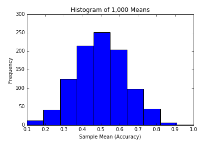
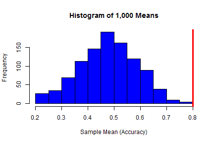
## Let's pretend that we know Han's accuracy is 50% ## and let's also randomly generate 10,000 shots numberOfShots = 10**4 import random as rd ## set the seed so we can reproduce our results rd.seed(162534) ## define function that generates 10 random shots def shotGenerator(numShots): tenShots = [] for i in range(numShots): if rd.random() < 0.50: tenShots.append(0) else: tenShots.append(1) return tenShots ## create a list of 1,000 lists of 10 random shots each simulatedShots = [shotGenerator(10) for x in xrange(numberOfShots/10)] ## create a list of means of each group of 10 shots means = [] for row in simulatedShots: means.append(float(sum(row))/len(row)) ## make histogram of means, see which accuracy levels are most common import matplotlib.pyplot as plt plt.hist(means) plt.title("Histogram of 1,000 Means") plt.xlabel("Sample Mean (Accuracy)") plt.ylabel("Frequency") plt.show() |
|
1 2 3 4 5 6 7 8 9 10 11 |
## note that histograms and p values will differ between R and Python, ## due to the different random number generators they use ## count the number of fights where Han's accuracy was at least 80% ## and divide by the total number of fights ## This gives the p value, ## the probability of observing an accuracy of at least 80%, ## assuming that Han's overall accuracy is actually 50% pValue <- length(means[means >= 0.8])/(numberOfShots/10) print(pValue) |
|
1 2 3 4 5 6 7 8 9 10 11 12 13 14 15 16 |
## note that histograms and p values will differ between R and Python, ## due to the different random number generators they use ## count the number of fights where Han's accuracy was at least 80% count = 0 for mean in means: if mean >= 0.8: count += 1 ## Divide the number of fights where Han's accuracy was at least 80% ## by the total number of fights. This gives the p value, ## the probability of observing an accuracy of at least 80%, ## assuming that Han's overall accuracy is actually 50% pValue = float(count) / len(means) print(pValue) |
|
1 |
0.059 |
|
1 |
0.053 |
|
1 2 3 |
## the portion of the blue to the right of the red line ## is the p-value, the probability of observing 80% or ## greater accuracy, assuming the true accuracy is 50% |
|
1 2 3 |
## the portion of the blue to the right of the red line ## is the p-value, the probability of observing 80% or ## greater accuracy, assuming the true accuracy is 50% |
|
1 2 3 4 5 |
hist(means, col = "blue", main = "Histogram of 1,000 Means", xlab = "Sample Mean (Accuracy)") abline(v = 0.8, lwd = 3, col = "red") |
|
1 2 3 4 5 6 |
plt.hist(means) plt.axvline(x=0.8, linewidth = 3, color = 'r') plt.title("Histogram of 1,000 Means") plt.xlabel("Sample Mean (Accuracy)") plt.ylabel("Frequency") plt.show() |
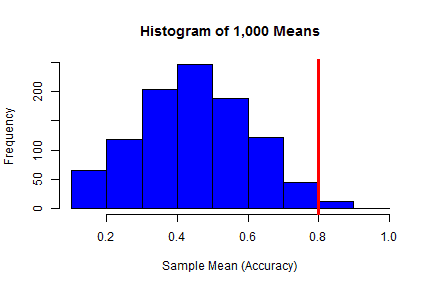
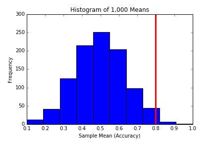
So based on the simulation’s results, the probability of Han shooting with 80% accuracy or more over 10 shots is 5.9% (based on R’s random number generation), or 5.3% (based on Python’s random number generation), assuming that Han’s real accuracy (the accuracy he exhibits over the long term) is 50%. Rey realizes that this suggests Han’s accuracy is higher than 50%, though probabilities of 5.9% and 5.3% are still too high to let Rey relax. After all, if Han’s accuracy is truly anywhere near 50% as Rey assumes, then they will easily be overwhelmed in the next wave.
But she doesn’t have time to ponder the odds any further, as the second group of troopers storm in, blasters blazing. Han had repositioned himself in the interim, and manages to catch the troopers by surprise. Three go down in a flash, and it’s another couple minutes before the last blaster sounds. Rey counts another 10 shots from Han’s blaster and 8 more Storm Troopers scattered across the battlefield. She can see another two in the distance running towards the hangar exit. In total then, there have been 16 hits and 4 misses…
|
1 2 3 |
shots <- c(rep(hit, 8), rep(miss, 2), rep(hit, 8), rep(miss, 2)) print(shots) print(mean(shots)) |
|
1 2 3 |
shots = [hit]*8 + [miss]*2 + [hit]*8 + [miss]*2 print(shots) print(float(sum(shots))/len(shots)) |
|
1 2 |
1 1 1 1 1 1 1 1 0 0 1 1 1 1 1 1 1 1 0 0 0.8 |
|
1 2 |
[1, 1, 1, 1, 1, 1, 1, 1, 0, 0, 1, 1, 1, 1, 1, 1, 1, 1, 0, 0] 0.8 |
…which gives the same accuracy as before of 80%. Updating the simulation with this new data,
|
1 2 3 4 5 6 7 8 9 10 11 12 13 14 15 |
## now we have a sample of 20 shots, ## so we will simulate twice as many shots as before numberOfShots <- 2*(10^4) simulatedShots <- sample(c(hit, miss), numberOfShots, replace = TRUE, prob = c(accuracy, 1-accuracy)) groupsOf20 <- matrix(simulatedShots, nrow = numberOfShots/20, ncol = 20, byrow = TRUE) means <- apply(groupsOf20, 1, mean) hist(means) pValue <- length(means[means >= 0.8])/(numberOfShots/20) print(pValue) |
|
1 2 3 4 5 6 7 8 9 10 11 12 13 |
## now we have a sample of 20 shots, ## so we will simulate twice as many shots as before numberOfShots = 2*(10**4) simulatedShots = [shotGenerator(20) for x in xrange(numberOfShots/20)] means = [] for row in simulatedShots: means.append(float(sum(row))/len(row)) count = 0 for mean in means: if mean >= 0.8: count += 1 pValue = float(count) / len(means) print(pValue) |
|
1 |
0.004 |
|
1 |
0.003 |
|
1 2 3 4 5 |
hist(means, col = "blue", main = "Histogram of 1,000 Means", xlab = "Sample Mean (Accuracy)") abline(v = 0.8, lwd = 3, col = "red") |
|
1 2 3 4 5 6 |
plt.hist(means, bins = 13) plt.axvline(x=0.8, linewidth = 3, color = 'r') plt.title("Histogram of 1,000 Means") plt.xlabel("Sample Mean (Accuracy)") plt.ylabel("Frequency") plt.show() |
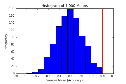
Rey breathes a sigh of relief. There is now merely a 0.4% or 0.3% chance of Han having exhibited 80% accuracy when his true long term accuracy is 50%, meaning his accuracy is almost certainly higher. She leans against the wall of the hangar and watches as Han Solo proves all the stories to be true during the next 2 waves of troopers. Let’s get the hell out of here kid, says Han.
So from the simulation, we were able to reject the hypothesis that Han Solo’s accuracy is 50%. But in what range of accuracy values can we expect his accuracy to lie? Do we know for sure his accuracy is 80%? Or perhaps we should only expect it to be somewhere between 70% and 90%? Or maybe a wider range, such as 60% to 100%? This is the topic of confidence intervals, which will be covered in a later post.
Leave a comment